Note
This technote is not yet published.
Scheduling simulations currently use ESO’s skycalc software to pre-calculate sky brightness for the survey. The current storage format, healpix maps of the sky sampled every few minutes, results in inconveniently large files of cached data. Here, I present an exploration of the use of Zernike polynomial coefficients as an alternative.
1 Summary
- Sky brightness is diffuse light spread across the field of view of the camera.
- Sky brightness includes components from emission from the atmosphere, scattered light from various source (the Moon, Sun, etc.), and Zodiacal light.
- Sky brightness varies smoothly over the sky, except near the moon. See Figure 1.
- Sky brightness varies slowly with time, except when the moon is rising or setting.
- The Rubin Observatory scheduler requires an estimate of the foreground sky brightness over the visible sky at each time for which it schedules exposures.
- The limiting magnitude (which depends on sky brightness) is one of the “features” the feature-based scheduler uses to order candidate exposures.
- When Poisson noise from the sky background is the dominant source of noise, the error in limiting magnitude due to an error in sky brightness (in magnitudes/asec^2) is half the error in sky brightness. For example, an uncertainty of 0.2 magnitudes in sky brightness corresponds to an uncertainty of 0.1 magnitudes in limiting magnitude.
- The current version of the scheduler uses a look-up table of sky values.
- The Rubin Obs. scheduler looks up sky brightness values in a set of healpix (nside=32) sky maps, for each of the six filters, at 5 to 15 minute time steps from 2022-09-01 to 2037-09-04 (excluding daytime). These healpix maps are created using interpolation of sample points produced by skycalc.
- skycalc is a sky brightness model written for the exposure time calculator used by the European Southern Observatory’s (ESO) Very Large Telescope (VLT) at Cerro Paranal.
- Sky brightness in each Rubin Observatory filter are generated by integrating the modeled SED over the corresponding instrument transmission curves.
- The full set of healpix maps occupy 144 GiB of disk space.
- Approximations of the sky brightness maps can be saved compactly using a Zernike transform.
- Zernike polynomials form a set of orthogonal basis functions on the unit disk. See Figure 2.
- Low order terms of a Zernike transform can approximate smoothly varying functions over the unit disk.
- Residuals between the pre-computed healpix maps and their approximation with a 6th order (27 term) Zernike approximation have a standard deviation of between 0.006 and 0.014 in all bands, much less than the standard deviation of the residuals between the skycalc model and the observed sky: typical uncertainty in the residuals is not significant compared to the uncertainty of \(\sim 0.2\) in the model itself.
- The residuals do not follow a normal distribution; the distribution has narrow tails extending from -0.27 magnitudes to 0.12 magnitudes. See Figure 6.
- The extreme tails in the residuals occur near the moon, when the moon is itself at high airmass. See Figure 8, Figure 9, and Figure 10.
- The
lsst.sims.sky_brightness_pre.zernikepython module provides an interface for use of Zernike coefficients to store sky brightness. This module:- uses coefficients stored in an
hdf5file with a size of 294 MiB (for coefficients up to 6th order); - interpolates Zernike coefficients for times not exactly covered by the original set of healpix maps; and
- provides an API similar to that of
lsst.sims.sky_brightness_pre.SkyModelPre, but does not include options no longer needed by current versions of the scheduler.
- uses coefficients stored in an
2 Background
The Legacy Survey of Space and Time (LSST) is an imaging sky survey which will be performed using the Vera C. Rubin Observatory, currently under construction. Exposure scheduling, the selection of which pointings on the sky to image at which times, will be automated by the Rubin Observatory automated scheduler. This scheduler selects exposures using a feature-based Markov decision process: at the time an exposure (or set of exposures) needs to be scheduled, the scheduler calculates a set of values (“features”) for each filter, over the visible sky. Using a linear combination of these features, the scheduler then calculates a score (the “reward function”) that represents how good it is to perform exposures in that band and that pointing and desired time, and selects exposures to maximize the reward. The three most important features used by the scheduler are (in simplified form):
- The slew time: the amount of time “lost” in overhead due to repointing the telescope.
- Survey progress: the difference between the number of already completed exposures (at each pointing, in each band) and the number desired (for the current time).
- The difference between the predicted point source \(5\sigma\) limiting magnitude (at each pointing, in each band) and the \(5\sigma\) in dark time on the meridian (for that pointing and band).
The third feature in this list is a measure of the expected data quality: the faintness of objects whose brightnesses can be measured to a reference precision. There are two dominant factors that influence the limiting magnitude: the point spread function (the sharpness of the image), and the noise in the image. The dominant factor in the noise relevant to objects near the magnitude limit is from statistical uncertainty in the light that covers the same pixels as the image of the object, but is not from the object being measured. For isolated point sources, this is from “sky brightness”, diffuse light that covers the entire image. Estimation of the sky brightness is therefore essential for the predicting the limiting magnitude, which is required to calculate the reward function, and therefor for selection of exposures by the scheduler.
Sky brightness arises from a variety of sources, including:
- airglow, light emitted by the Earth’s upper atmosphere from a variety of causes, including recombination of atoms photo-ionized by the Sun;
- twilight, sunlight scattered by the Earth’s atmosphere when the Sun is just under the horizon;
- starlight and moonlight scattered by the Earth’s atmosphere;
- Zodiacal light, sunlight scattered by dust in the plane of our solar system; and
- light pollution, light from terrestrial sources scattered by the Earth’s atmosphere.
Krisciunas & Schaefer (1991) [3] describe a simple model for estimating using a highly simplified model: airglow from a thin spherical shell in the atmosphere, and single scattering of moonlight in the atmosphere. The Dark Energy Survey (DES) scheduler used a refinement of this model, plus a rough model for twilight, to estimate the sky brightness to between 0.2 and 0.3 \(\frac{\textrm{mag}}{\textrm{asec}^2}\), depending on the band, for dark and moony skies outside of twilight. (Bluer bands had lower residuals.) ESO’s skycalc software improves on this model in several ways, estimating the full spectral energy distribution of the sky brightness using physical models for atmospheric processes that result in airglow, multiple scattering of starlight and moonlight, and a model for Zodiacal light. These improvements result in a model that estimates the sky brightness with residuals of 0.2 \(\frac{\textrm{mag}}{\textrm{asec}^2}\) across all bands (Jones et al. 2013 [2]).
3 The Current System
Each time the scheduler selects an exposures (or set of exposures), it evaluates the reward function across the sky, sampled at (nside=32) Healpix healpixel locations (in equatorial coordinates) at the time for which exposures need to be chosen. It therefore needs values for sky brightness estimates on these sample points, as a function of time.
It is impractical to use the skycalc software to calculate these values on demand. Instead, the scheduling team used skycalc to calculate the various components (airglow, scattered moonlight, Zodiacal light, scattered starlight, and atmospheric emission lines) of the sky brightness over relevant ranges of paramaters (airmass, position and phase of the moon, etc.). These components are then interplated and combined to form overall sky brightness maps at each sample point over a set of sample times. These sample times occur every 5 to 15 minutes for each night between 2022-09-01 and 2037-09-04, covering the full date range of LSST. These data are saved in a set of files totaling 144 GiB. When evaluating the reward function, the scheduler looks up the pre-computed sky brightness values near the desired times, and interpolates for the desired time. See Yoachim et al. (2016) [1] for further details.
Figure 1 shows examples of sky brightness maps calculated following this procedure, for times when the moon is down (so the sky brightness is dominated by airglow), and when the moon is near full and above the horizon (so scattered moonlight is a major contributor to sky brightness). In both cases, the sky brightness varies smoothly. The sharpest variation occurs where the sky is brightest: near the moon, and just above the maximum airmass: locations on the sky the scheduler will avoid anyway.
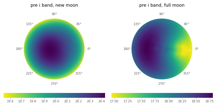
Figure 1 Sky brightness maps of the sky brightness as stored in the cached healpix map files, generated using skycalc. The color scales are in units of \(\frac{\textrm{mag}}{\textrm{asec}^2}\). The maps are in horizon coordinates: the center of each map is the zenith, and the radial coordinate the angle with zenith (with a maximum zenith distance of \(69^{\circ}\)).
The Rubin Observatory scheduler calls its sky brightness estimator by passing a time (as a floating point MJD) and set of healpix coordinates, which returns a dictionary of numpy arrays of sky brightness values.
The keys of this dictionary are the filters, and the values are arrays that hold the sky brightness values (corresponding to the array of indices provided).
>>> import numpy as np
>>> import healpy
>>> from lsst.sims.skybrightness_pre import SkyModelPre
>>>
>>> mjd = 59854.3
>>> npix = 32
>>>
>>> ra1, decl1 = 0, -50
>>> pointing1 = healpy.ang2pix(npix, ra1, decl1, lonlat=True)
>>>
>>> ra2, decl2 = 0, -20
>>> pointing2 = healpy.ang2pix(npix, ra2, decl2, lonlat=True)
>>>
>>> healpix_idxs = np.array((pointing1, pointing2))
>>>
>>> sky_model_pre = SkyModelPre()
>>> sky_brightness = sky_model_pre.returnMags(mjd, healpix_idxs)
>>>
>>> print("Sky brightness in i at pointing 1:",  sky_brightness['i'][0])
Sky brightness in i at pointing 1: 20.211941485692027
>>> print("Sky brightness in g at pointing 2:",  sky_brightness['g'][1])
Sky brightness in g at pointing 2: 21.908871333901892
If no healpix ids are provided in the call to returnMags, then the array of sky values over the whole sphere is returned, and the healpix ids are the indices of the array.
4 Justification and scope of changes
The current method of storing the sky brightness values is inconveniently and unnecessarily large: a full nside=32 healpix map (pre-computed for each time sample) stores the sky brightness for 12288 sample pointings, at high precision. The sky brightness, however, varies slowly as a function pointing for most locations on the sky, and the model is only good to a precision of 0.2 \(\frac{\textrm{mag}}{\textrm{asec}^2}\).
The scope of this proposal is limited to replacing the use of storage of pre-computed sky values by the scheduler with a more compact approximation. It does not propose to change the underlying physical model used, nor calculation of sky brightness in any context outside of the scheduler itself.
5 The Proposed System
5.1 Background: Zernike polynomials as basis functions
As approximations of smoothly varying functions on the unit disk that show significant radial symmetry, Zernike coefficients are a promising candidate. Zernike polynomials form a set of orthogonal basis functions on the unit disk. This use of Zernike polynomials is directly analogous to simple Fourier-transform based lossy image compression techniques, but is more naturally applied to the unit disk, and particularly suitable for functions with rotational symmetry. In the simplest applications, the transform can be truncated to include only lower order terms. Such a truncation has the effect of blurring the image. In more sophisticated applications, terms near zero can be set to zero and the result compressed. The same approaches can be applied using the Zernike transform as well. Because the “image” being compressed is smoothly varying, only a simple truncation is explored here (although the more sophisticated approach may be useful).
There are several conventions for indexing and normalizing Zernike polynomials. Those used here are from Thibos et al. (2002) [4]:
where
and
Here, \(\delta\) is the Kronecker delta, \(m\) is the angular frequency of the term, and \(n\) the radial order. For a given radial order n, the angular frequency can have values \(-n, -n+2, -n+4, ..., n\). For the purposes of storing values and coefficients in a single dimensional array, it is convenient to define a single index, the mode number:
Zernike coefficients that fit a function on the unit disk (the values of the Zernike transform of the function) are then:
Figure 2 shows \(Z^{m}_n(\rho,\phi)\) graphically, and provides some intuition for the kinds of functions low order Zernike coefficients can effectively represent.
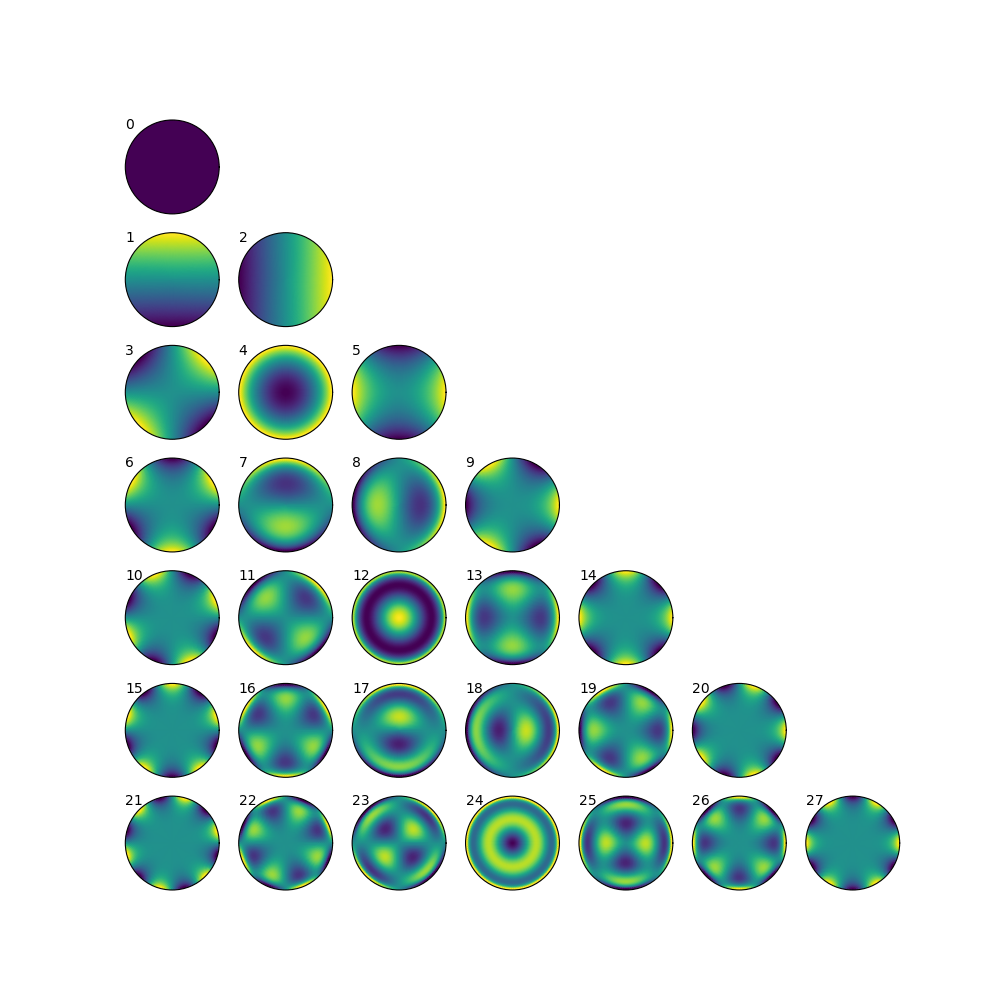
Figure 2 The Zernike polynomials, \(Z^{m}_n(\rho,\phi)\), for \(n<7\). The number to the upper left of each subplot shows the mode number, \(j\) (the single-valued index).
5.2 Implementation
5.2.1 Computation from Zernike coefficients and polynomials
To compute estimates of the sky brightness, the lsst.sims.skybrightness_pre.zernike.ZernikeSky class evaluates
\(t\) represents the time (stored as an MJD), and \(\rho, \phi\) the coordinates in the disk over which the Zernike polynomials are orthogonal.
As used in the ZernikeSky class, \(\phi\) is the azimuthal angle in horizon coordinates, and \(\rho = \frac{\mathrm{zd}}{\mathrm{zd_{max}}}\), where zd is the angular zenith distance, and zd max the maximum zenith distance for which surface brightness is to be calculated.
The mode number, \(j\), is used here rather that the more traditional radial order and angular frequency indices (\(n, m\)) to simplify storage in a pandas.DataFrame or numpy array.
The sum contains two components: the coefficients, \(c[j](t)\), and the values of the Zernike polynomial themselves, \(Z[j](\rho,\phi)\).
The values of the coefficients for a given mode number is a function only of time, not location on the sky, while the values of the Zernike polynomials (for a given mode number) are a function only of the location on the sky (in horizon coordinates).
To implement the API shown above, the Zernike-based sky brightness code requires values of \(c[j]\) at the mjd requested, and \(Z[j](\rho,\phi)\) for each healpix index requested.
5.2.2 Estimation of Zernike coefficients \(c[j](t)\)
The ZernikeSky.load_coeffs method reads values for the Zernike coefficients from an hdf5 file into a pandas.DataFrame, with columns for each Zernike mode number and rows for each time step fit, such that each row corresponds to a time at which the lsst.sims.skybrightness_pre.SkyModelPre stores a full healpix map.
Each (nside=32) healpix map contains 12288 values, while a row in the pandas.DataFrame of Zernike coefficients though a radial degree of 6 has 28 values, a factor of \(\sim 439\) times more compact.
Figure 3 shows the variation in the values of the Zernike coefficients over time, over the course of a dynamic night.
At the end of evening twilight, the moon is below the horizon, but rises shortly thereafter.
The effect is particularly clean in the \(Z_0^0\) term, in which the sky brightness drops sharply at the start of the night (evening twilight), briefly plateaus (the portion of the night during which the moon is below the horizon), the brightens as the moon rises.
Over the course of the night, the moon rises into the area covered by the sky approximation, transits, and begins to set.
It can be seen from the plots that the contribution of each Zernike polynomial drops as the radial order increases, with the lowest order terms having the most significant influence on the calculated sky brightness.
It can also be seen that, except at the precise time step at which the moon rises, the values of the coefficients vary smoothly with time relative to the sampling in time: values of coefficients between points can be effectively estimated by simple linear interpolation.
This is what the lsst.sims.skybrightness_pre.zernike.ZernikeSky class does.
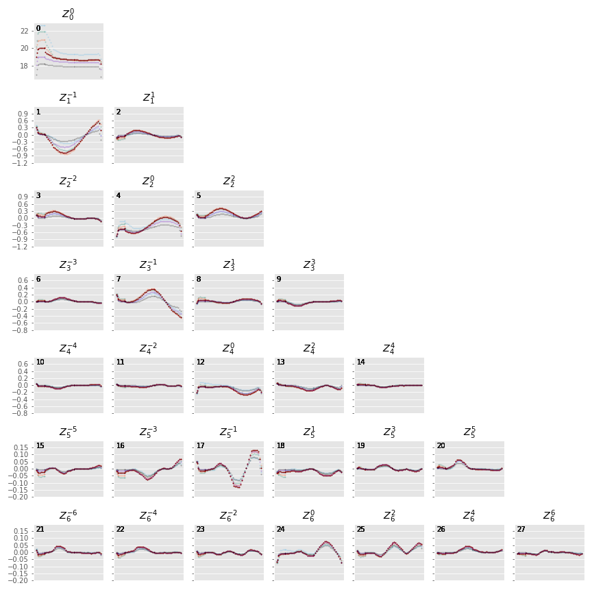
Figure 3 The values of the Zernike coefficients for a particularly dynamic night, in which the moon begins beneath the horizon and then rises and transits over the course of the night. The coefficients are scaled such that the values on the vertical axis represent the maximum change in magnitude contributed by each mode number. The heavy red points show the values for i band, while the fainter points in other colors represent other filters.
5.2.3 Estimation of Zernike polynomial values \(Z[j](\rho, \phi)\)
While the coefficients themselves are functions of the time and independent of the location on the sky, the values of the Zernike polynomials of a given mode number are themselves functions only of the location on the sky (in horizon coordinates).
Each \(Z_m^n(\rho, \phi)\) term is the product of a polynomial in \(\rho\) and a trigonometric function of \(\phi\), making it the most computationally expensive requirement for calculating the \(F(t, \rho, \phi)\).
The values, however, of \(Z_m^n(\rho, \phi)\) do not change with time.
If we are making repeated calculations at specific values of \(\rho, \phi\), these values can be computed once and cached.
To fulfill the API, ZernikeSky must provide sky brightness values at a predefined set of coordinates, suggesting that we can simply calculate \(Z_m^n\) at these values, but there is a problem: the healpix coordinates in the argument are predefined in equatorial coordinates, but the values of \(Z_m^n\) are constant in horizon coordinates.
The values of \(\rho, \phi\) for the given set of healpix values are a function of the local Sidereal time (LST), so the values of \(Z_m^n\) are as well.
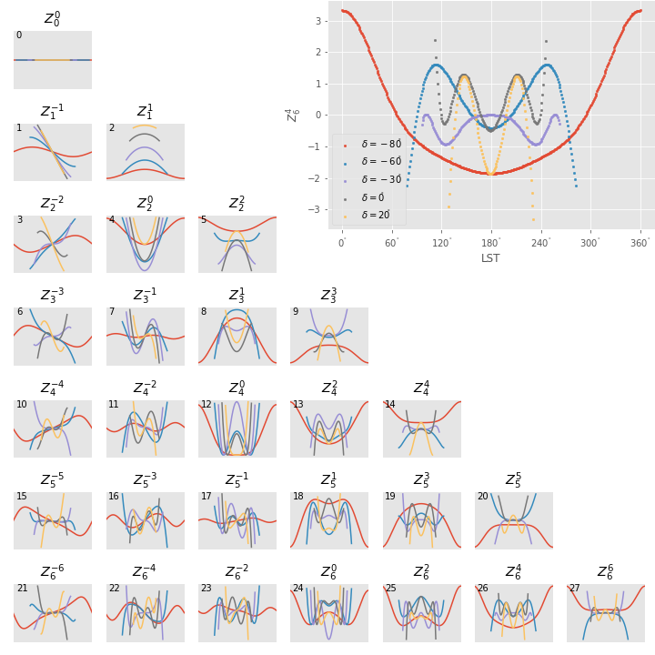
Figure 4 The variation of \(Z_m^n\) as a function of LST for several sample equatorial healpixels at different declinations. (Variation in R.A. shifts the values horizontally, but does not affect the shape of the curves.) Sidereal times for which the curves have no values shown are time at which these pointings are at a zenith distance greater than the range of the Zernike function. The lowest order functions (shown in the upper rows) correspond to Zernikes that have the greatest influence on the ultimate sky brightness estimate (see corresponding plots in Figure 3), have Zernike polynomials that vary most smoothly over the sky (Figure 2), and have the smoothest behavior in this plot.
Rather than calculate \(Z_m^n(\rho, \phi)\) “from scratch” for each healpix at the time requested, ZernikeSky pre-computes Z[j][hpix] at sequences of LST values for each Zernike mode number and equatorial healpixel, and interpolates to obtain the value of Z[j][hpix] at the LST corresponding to the MJD with which it is called.
The inset in the upper left of Figure 4 shows sampled points for five different healpixels and different declinations.
5.2.4 Computing sky brightness with ZernikeSky
To calculate the sky brightness using an API that following that used by the scheduler:
>>> import numpy as np
>>> import healpy
>>> from lsst.sims.skybrightness_pre.zernike import SkyModelZernike
>>>
>>> mjd = 59854.3
>>> npix = 32
>>>
>>> ra1, decl1 = 0, -50
>>> pointing1 = healpy.ang2pix(npix, ra1, decl1, lonlat=True)
>>>
>>> ra2, decl2 = 0, -20
>>> pointing2 = healpy.ang2pix(npix, ra2, decl2, lonlat=True)
>>>
>>> healpix_idxs = np.array((pointing1, pointing2))
>>>
>>> sky_model = SkyModelZernike()
>>> sky_brightness = sky_model.returnMags(mjd, healpix_idxs)
>>>
>>> print("Sky brightness in i at pointing 1:",  sky_brightness['i'][0])
Sky brightness in i at pointing 1: 20.240004108584117
>>> print("Sky brightness in g at pointing 2:",  sky_brightness['g'][1])
Sky brightness in g at pointing 2: 21.967150461105156
This example relies on finding the hdf file with the Zernike coefficients in ${SIMS_SKYBRIGHTNESS_DATA}/zernike/zernike.h5.
If it is located elsewhere, the first argument in the instantiation of SkyModelZernike should be the path to this file.
5.3 Analysis
To test the effectiveness of approximating the pre-computed healpixel sky brightness values (interpolated from skycalc samples) using truncated Zernike transforms, I fit Zernike coefficients through the 5th (21 terms), 6th (27 terms), and 11th (78 terms) orders to each of these sampled time steps. Masked values in the healpix maps (around the zenith and moon) results in an unevenly sampled starting data set, so a least squares fit was used to derive the coefficients rather than a traditional sum of products.
Figure 5 and Figure 6 show typical pre-computed healpixel maps, their 6th order (27 term) Zernike approximation, and residuals for dark (moon below the horizon) and bright (full moon above the horizon) sample times. The residuals show high-frequency patterns not representable by Zernike functions of this order; compare the lower left subplots of these figures with the basis functions in Figure 2.
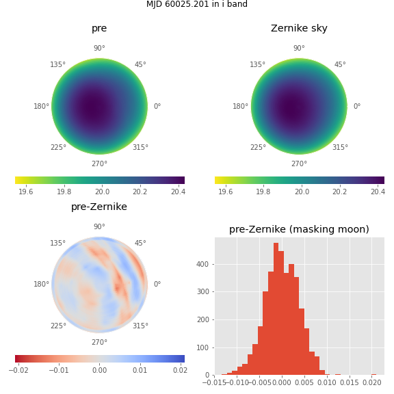
Figure 5 The upper two panels show the sky brightness values at sampled healpixels (pre-computed by interpolated skycalc values) for a typical fully dark (no moon) time (in horizon coordinates, with zenith at the center) on the left, and the Zernike approximation of these values on the night. The lower left figure shows the difference between the pre-computed sky brightness and its Zernike approximation, and the lower right histogram shows the distribution of these residuals, masking the \(20^{\circ}\) around the moon.
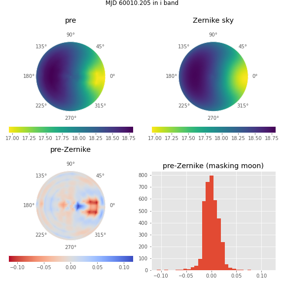
Figure 6 The subplots above have the same meaning as those in Figure 5, except for a time with a full moon above the horizon.
The distribution is dominated by residuals less than 0.05 magnitudes in all cases, but thin tails extend from \(\sim -0.25\) to \(\sim 0.15\). The quantiles and extreme of residuals for areas of the sky considered by the schuduler (greater than \(\sim 30^{\circ}\) from the moon) are as follows:
| order | band | mean | std | min | 0.01% | 0.1% | 1% | 50% | 99% | 99.9% | 99.99% | max |
|---|---|---|---|---|---|---|---|---|---|---|---|---|
| 6th | u | 0.00 | 0.02 | -0.14 | -0.12 | -0.10 | -0.04 | -0.00 | 0.04 | 0.06 | 0.08 | 0.10 |
| 6th | g | 0.00 | 0.02 | -0.26 | -0.16 | -0.11 | -0.05 | -0.00 | 0.05 | 0.08 | 0.12 | 0.17 |
| 6th | r | 0.00 | 0.02 | -0.24 | -0.15 | -0.11 | -0.05 | -0.00 | 0.05 | 0.08 | 0.10 | 0.14 |
| 6th | i | 0.00 | 0.02 | -0.17 | -0.13 | -0.10 | -0.04 | -0.00 | 0.05 | 0.06 | 0.09 | 0.13 |
| 6th | z | 0.00 | 0.01 | -0.15 | -0.12 | -0.09 | -0.04 | -0.00 | 0.04 | 0.06 | 0.08 | 0.12 |
| 6th | y | 0.00 | 0.01 | -0.13 | -0.12 | -0.09 | -0.03 | -0.00 | 0.04 | 0.06 | 0.07 | 0.08 |
| 7th | u | -0.00 | 0.01 | -0.11 | -0.06 | -0.05 | -0.02 | -0.00 | 0.02 | 0.04 | 0.05 | 0.07 |
| 7th | g | -0.00 | 0.01 | -0.23 | -0.13 | -0.08 | -0.03 | -0.00 | 0.03 | 0.06 | 0.09 | 0.12 |
| 7th | r | -0.00 | 0.01 | -0.20 | -0.12 | -0.07 | -0.03 | -0.00 | 0.03 | 0.06 | 0.08 | 0.11 |
| 7th | i | -0.00 | 0.01 | -0.14 | -0.08 | -0.05 | -0.02 | -0.00 | 0.03 | 0.05 | 0.08 | 0.12 |
| 7th | z | -0.00 | 0.01 | -0.09 | -0.05 | -0.04 | -0.02 | -0.00 | 0.02 | 0.04 | 0.06 | 0.10 |
| 7th | y | -0.00 | 0.01 | -0.06 | -0.05 | -0.04 | -0.02 | -0.00 | 0.02 | 0.03 | 0.05 | 0.08 |
| 12th | u | 0.00 | 0.00 | -0.07 | -0.04 | -0.03 | -0.01 | 0.00 | 0.01 | 0.04 | 0.06 | 0.10 |
| 12th | g | 0.00 | 0.01 | -0.14 | -0.07 | -0.04 | -0.02 | 0.00 | 0.02 | 0.06 | 0.09 | 0.13 |
| 12th | r | 0.00 | 0.01 | -0.12 | -0.07 | -0.04 | -0.02 | 0.00 | 0.03 | 0.07 | 0.09 | 0.13 |
| 12th | i | 0.00 | 0.01 | -0.08 | -0.05 | -0.03 | -0.01 | 0.00 | 0.02 | 0.06 | 0.09 | 0.12 |
| 12th | z | 0.00 | 0.00 | -0.07 | -0.03 | -0.02 | -0.01 | 0.00 | 0.02 | 0.05 | 0.08 | 0.10 |
| 12th | y | 0.00 | 0.00 | -0.04 | -0.02 | -0.02 | -0.01 | 0.00 | 0.01 | 0.03 | 0.06 | 0.08 |
Figure 7 shows the histograms of the residuals for each order tested, in each filter, for the first year of tested data. The log scale accentuates the long tails of the distribution. Recall that the standard deviation of the residuals of the skycalc model with respect to actual data is \(\sim 0.2\): instances where the the difference between the Zernike approximation and the skycalc value are comparable to the precision of the skycalc model are rare, but they exist.
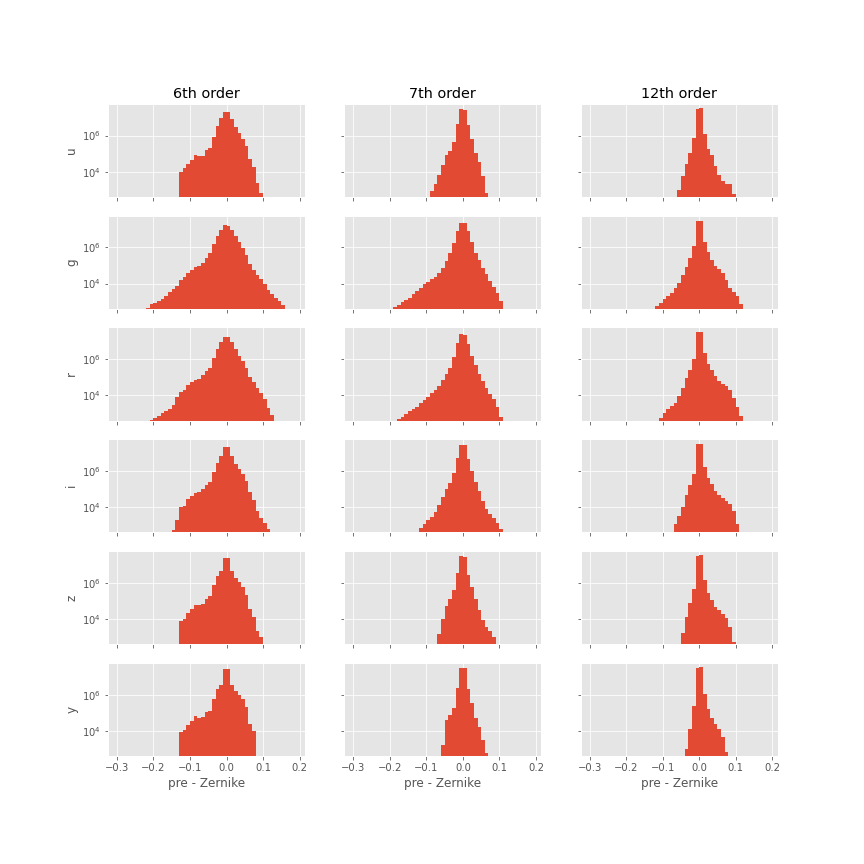
Figure 7 Histograms of the differences between the precomputed healpixel sky brightness and their Zernike approximation, on a log scale, for all filters and with Zernike approximations to 5th, 6th, as 11th order. Note the log scale covering 7 orders of magnitude: the distribution is sharply peaked around 0.
Examination of examples of time samples with bad residuals indicate conditions under which Zernike approximations perform most poorly. Figure 8 shows the maps, residuals, and histogram of residuals for the worst time step in the first year. It occurs when the moon is at an altitude of \(\sim 20^{\circ}\), just outside the area covered by the map (which extends only to a zenith distance of \(67^{\circ}\)). The worst residuals occur at the same azimuth as the moon: just above the moon on the sky.
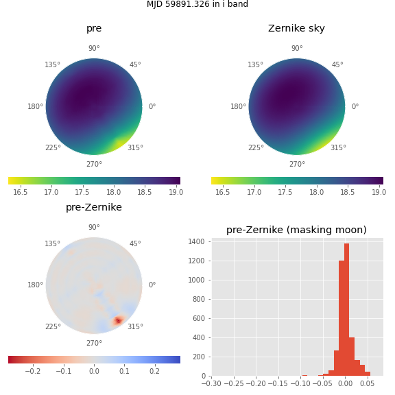
Figure 8 The subplots above have the same meaning as those in Figure 5, except for the time with the worst residuals.
Figure 9 and Figure 10 indicate that this is typical of the worst time steps: they occurr when the moon has an altitude of \(\sim 20^{\circ}\), in sky within \(\sim 20^{\circ}\) of the moon, and an altitude of less than \(\sim 40^{\circ}\). Note that the scheduler currently avoids pointings within \(\sim 30^{\circ}\) of the moon, regardless of sky brightness.
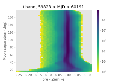
Figure 9 A 2-dimensional histogram of the sky estimates as a function of residual between pre-computed healpixel map magnitude and its Zernike approximation, and the angular separation between the point on the sky and the moon. The color is coded according to a log scale, covering 6 orders of magnitude. Note that the worst residuals are within \(20^{\circ}\) of the moon, while the scheduler avoinds pointings within \(\sim 30^{\circ}\) of the moon, regardless of sky brightness.
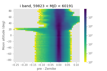
Figure 10 A 2-dimensional histogram of the sky estimates as a function of residuals between pre-computed healpixel map magnitudes and their Zernike approximation, and the altitude of the moon.. The color is coded according to a log scale, covering 6 orders of magnitude. Note that the worst residuals occur when the moon is at an altitude of about \(20^{\circ}\).
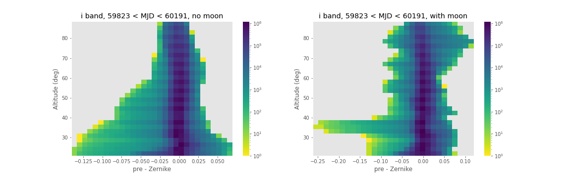
Figure 11 A 2-dimensional histogram of the sky estimates as a function of residual between pre-computed healpixel map magnitudes and their Zernike approximation, and the altitude an the sky. The color is coded according to a log scale, covering 6 orders of magnitude. Note that the worst residuals occur at altitudes below \(40^{\circ}\) (an airmass of about 1.6).
Although these histograms confirm that the very worst residuals occur in situations similar to those shown in Figure 8, they also show some residuals as bad as \(\sim 0.15\) magnitudes occur even in dark time. Figure 12 shows the sample time with the worst residuals in dark time. The “spike” of brightness at an azimuth of \(\sim90^{\circ}\) is suggestive of zodiacal light, and indeed this time step is near twilight, with the sun azimuth near the area with high residuals (\(\mbox{az}=95^{\circ}\)), as one would expect if this were zodiacal light.
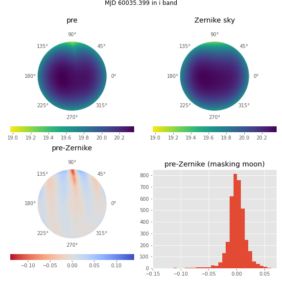
Figure 12 The subplots above have the same meaning as those in Figure 5, except for the dark time (moon below the horizon) with the worst residuals.
If zodiacal light is the cause of all of the extreme dark time residuals, then one would expect these high residuals only to occur at low ecliptic latitude, and indeed this is what Figure 13 shows.
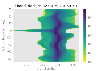
Figure 13 A 2-dimensional histogram of the sky estimates as a function of residual between pre-computed healpixel map magnitudes and their Zernike approximation, and the ecliptic latitude. The color is coded according to a log scale, covering 6 orders of magnitude. Note that the worst residuals occur at ecliptic latitudes close to 0.
6 Timing
The calculation of the Zernike sky requires computing the sums of Zernike coefficients, and therefore requires additional compute time over a simple look-up table. Testing on a lightly loaded system shows the following timings for the look-up table and Zernike approximation computation of the full set of healpixel values at one MJD:
| Method | Time (ms) |
|---|---|
| healpix | 4.5 |
| 5th order | 9.8 |
| 6th order | 11.9 |
| 11th order | 24.3 |
7 Conclusion and future work
Replacement of the healpix look-up table based storage of sky brightness values with one based on approximations using fit Zernike coefficients will have the following effects:
- The disk storage required for the sky brightness data will drop from 144GiB to 220 MiB (for 5th order), 294 MiB (for 6th order), or 811 MiB (for 11th order).
- The values returned will not be exactly those calculated by skycalc, but only approximations with residuals with standard deviations of \(0.02~\mbox{mag/asec}^2\) in all cases, and rare extreme deviations of up to 0.26, 0.23, or 0.17 \(\mbox{mag/asec}^2\) for 5th, 6th, and 11th order Zernike polynomials, respectively. These extreme deviations occur near a bright moon, when the moon is at an altitude of \(\sim20^{\circ}\). For comparison, the precision of the model is about \(0.20~\mbox{mag/asec}^2\).
- The time required for the schedule to obtain sky brightness values increases by 77%, 122%, and 448% for 5th, 6th, and 11th order Zernikes, respectively.
There are additional optimizations that can be made to reduce the disk space required. Figure 3 shows that the coefficients change only slowly with time relative to the current sampling: the coefficients can potentially be stored much more sparsely with little loss of precision. Furthermore, the limited precision of the model means that double precision data type with which the coefficients are stored may be excessive: the coefficients could potentially be stored as short floats without loss of effective precision.
8 Acknowledgements
This manuscript has been authored by Fermi Research Alliance, LLC under Contract No. DE-AC02-07CH11359 with the U.S. Department of Energy, Office of Science, Office of High Energy Physics.
References
| [1] | Peter Yoachim, Michael Coughlin, George Z. Angeli, Charles F. Claver, Andrew J. Connolly, Kem Cook, Scott Daniel, Željko Ivezić, R. Lynne Jones, Catherine Petry, Michael Reuter, Christopher Stubbs, and Bo Xin. An optical to IR sky brightness model for the LSST. In Observatory Operations: Strategies, Processes, and Systems VI, volume 9910, 99101A. International Society for Optics and Photonics, July 2016. doi:10.1117/12.2232947. |
| [2] | A. Jones, S. Noll, W. Kausch, C. Szyszka, and S. Kimeswenger. An advanced scattered moonlight model for Cerro Paranal. \aap , 560:A91, December 2013. arXiv:1310.7030, doi:10.1051/0004-6361/201322433. |
| [3] | K. Krisciunas and B. E. Schaefer. A model of the brightness of moonlight. \pasp , 103:1033–1039, September 1991. doi:10.1086/132921. |
| [4] | Larry N. Thibos, Raymond A. Applegate, James T. Schwiegerling, Robert Webb, and VSIA Standards Taskforce Members. Vision science and its applications. Standards for reporting the optical aberrations of eyes. Journal of Refractive Surgery (Thorofare, N.J.: 1995), 18(5):S652–660, October 2002. |